UC SANTA CRUZ · 2021

Attitude Estimation Using Complementary Feedback Filter

Using cheap sensors in fusion to solve the problem of attitude estimation — combining a gyroscope, accelerometer, and magnetometer into an Attitude Heading Reference System (AHRS).

B.S. Robotics Engineering · Sensor Fusion · Dept. of Electrical and Computer Engineering

Sensor FusionAHRSDCMIMUComplementary FilterMPU9250

DOWNLOAD PDF

Abstract

Estimation of rotation about the Earth is a common problem in aviation and other fields. The advent of the smartphone pushed the field of estimating orientation into the commercial realm, requiring cheaper solutions to a usually expensive problem. This paper deeply investigates using cheap sensors in fusion to solve the problem of attitude estimation.

1. Introduction

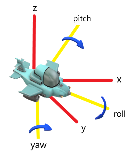
An AHRS (Attitude Heading Reference System) is the combination of several sensors to measure the rotation of an object relative to a global coordinate frame. Consider an aircraft — it becomes necessary to describe its heading: is it pointing straight down? Is it level with the surface of the Earth? The “attitude” of an object describes its rotation in respect to some reference frame.

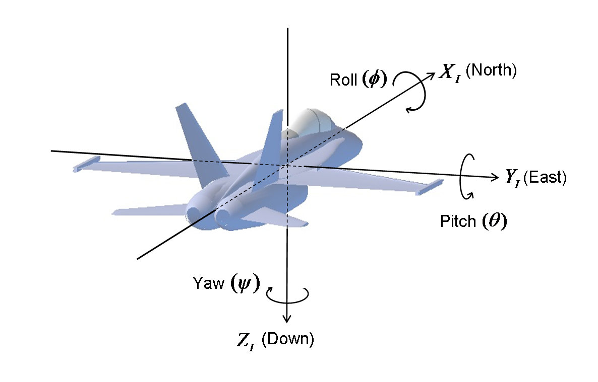
AHRS Measurements — Fig 1: AHRS measurements — Roll (φ), Pitch (θ), Yaw (ψ) relative to North/East/Down

1.1 Referencing Earth

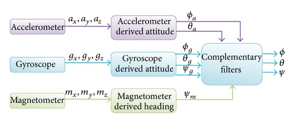
A magnetometer, accelerometer, and gyroscope sensor are used to create this system. The gyroscope is the primary sensor while the other two provide feedback. The accelerometer measures Earth's gravity and always has the information for “down,” and the magnetometer always points at North because of Earth's magnetic field.

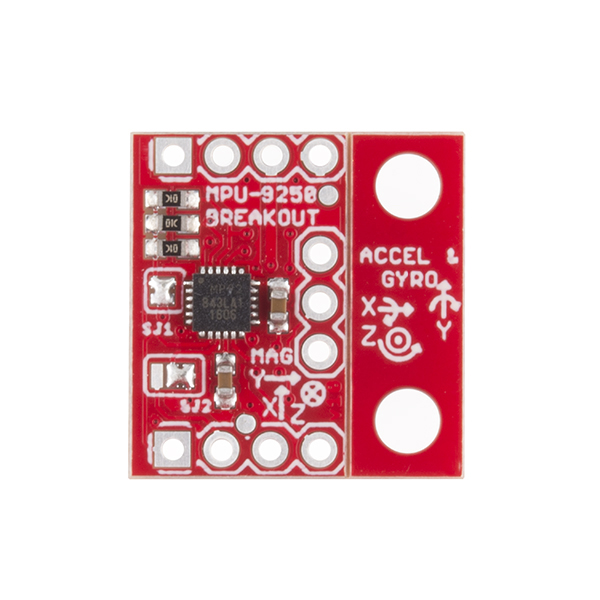
Fusion sensor diagram — Fig 2: Sensor fusion architecture — accelerometer, gyroscope, and magnetometer feed into complementary filters

1.2 MPU9250 Sensor

The MPU9250 breakout board by SparkFun was used, combining a gyroscope, magnetometer, and accelerometer in a single package with simple communication protocols.

MPU9250 board — Fig 3: MPU9250 breakout board by SparkFun

2. Storing the Rotation Angles

The rotation information is stored in a rotation matrix. Using linear algebra, this transformation matrix contains the relationship between the airplane's coordinate frame and the global coordinate frame:

R = R_yaw · R_pitch · R_roll
R : V⃗_plane → V⃗_global

This is referred to as the Direct Cosine Matrix (DCM) — standard nomenclature in attitude estimation.

Pitch, roll, yaw axes — Fig 4: Body frame axes — pitch, roll, and yaw

2.1 The DCM

The DCM is a 3×3 transformation matrix based on pitch (φ), roll (θ), and yaw (ψ) provided by the sensors. It contains all important information about the body frame and inertial frame, and is the transformation between the two. The inertial frame is based on cardinal directions (North, East, South, West), while the body frame is the perspective of the sensors.

The DCM connects spatial coordinates to angular ones. Matrix transformations are order dependent (ABC ≠ CBA). This implementation applies transformations in pitch, roll, yaw order — rotation around the x, y, then z axis.

3. Getting the Rotation Angles

Each sensor contributes different information to the attitude estimation:

ACCELEROMETER

Measures acceleration in x, y, z
Always measures gravity
Gives pitch and roll information
No yaw information

GYROSCOPE

Tracks rate of change of rotation
Integrate to get angle
Primary sensor in fusion
Tracks from starting position

MAGNETOMETER

Measures magnetic field
Always points to magnetic north
Gives yaw information
Affected by nearby magnets

4. Integration of Body-Fixed Rates

Two techniques convert gyro velocity data (deg/s) into rotation position data (deg): (1) forward integration and (2) matrix exponential form. Forward integration in matrix form is:

R⁺ = R⁻ + [ω⃗×]R⁻Δt

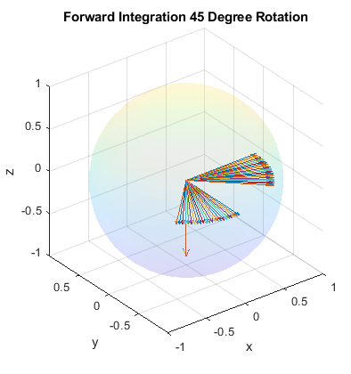
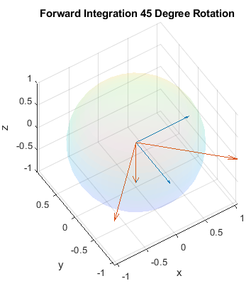
4.1 Forward Integration

Basic integration of gyro rotation rates using the skew symmetric ω matrix. With a simulated rotation rate of 1 deg/sec and polling rate of 1 Hz, the rotation appears stable for 45 degrees of rotation. However, the DCM doesn't maintain orthonormality over time — after nine revolutions, the x and y vectors are no longer unit vectors.

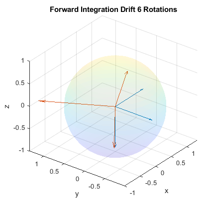
Simulated 45 degree rotation — Fig 5: Simulated 45° rotation

Drift after 9 revolutions — Fig 6: DCM drift — body frame vectors lose orthonormality after 9 revolutions

4.1.2 Experimental Forward Integration

Using real gyro data with previously determined biases and scale factor, the DCM drifts out of orthonormality after just 6 rotations in 30 seconds. This demonstrates that simple forward integration creates huge drifting errors in a short period of time.

Experimental drift 3D — Fig 7a: Experimental drift after 6 rotations (3D view)

Experimental drift norm — Fig 7b: Body frame vector norms diverge from 1.0 within 30 seconds

4.2 Rodrigues Rotation Matrix

The matrix exponential form maintains orthonormality of the DCM but still has errors relative to the gyro sensor in real space. The Rodrigues Exponential is:

R_exp(ωΔt) = I + sinc(ωΔt_norm) · cos(ωΔt_norm) · ωΔt + sinc(ωΔt_norm)²/2 · (ωΔt)²

5. Closed Loop Integration

The gyro sensor has no reference for the inertial frame — it only measures rotation from its starting position. The magnetometer and accelerometer provide absolute references: the accelerometer gives “down” (via gravity), and the magnetometer gives “north” (via Earth's magnetic field).

The closed loop uses two corrections: an error correction (corrects absolute angle of rotation for pitch and roll) and a bias estimate (accounts for systematic gyro bias that would otherwise overpower the error correction as values converge).

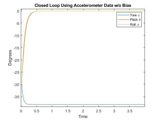
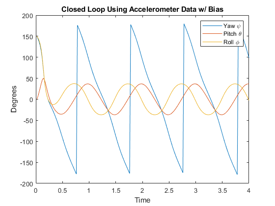
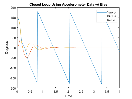
5.1 Z-Axis Error Correction

The error correction is calculated as wmeas_a = a⃗_b × R'a⃗_i, measuring the difference between the DCM and the accelerometer (which should always point down). Before integration, the error is added: ω⁺ = Kp_a · wmeas_a.

Without bias estimate, the pitch and roll converge toward the correct absolute rotations but cannot account for the bias error — as values get closer to correct, the error correction weakens and is overpowered by the bias. With the bias estimate B_estimate⁺ = −Ki_a · wmeas_a, pitch and roll level out and hold absolute positions even with bias.

Closed loop without bias — Fig 8: Without bias correction

With bias drift — Fig 9: With bias (uncorrected)

With bias corrected — Fig 10: With bias estimate — stable

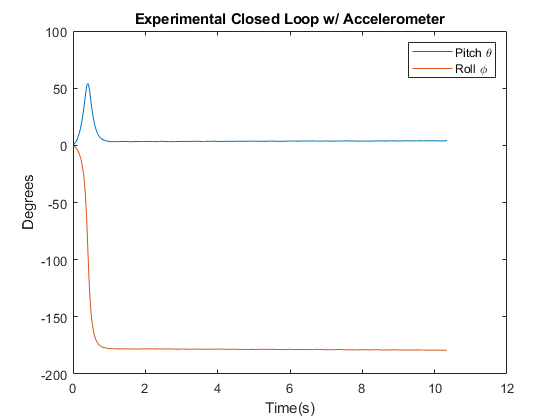
6. Accelerometer Feedback Tuning

The techniques were implemented on a microcontroller and compared to a MATLAB simulation. The proportional gain K_p was varied to determine the best noise-to-correction ratio. Higher K_p values reduce the time to acquire the initial position from ~15 seconds down to ~1 second.

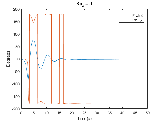
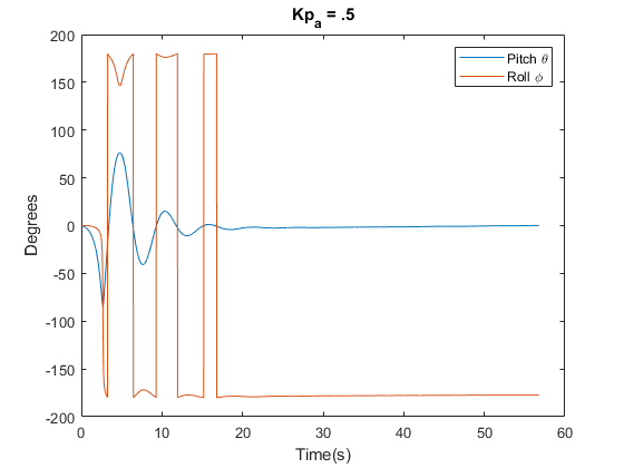
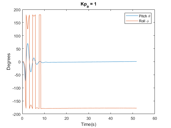
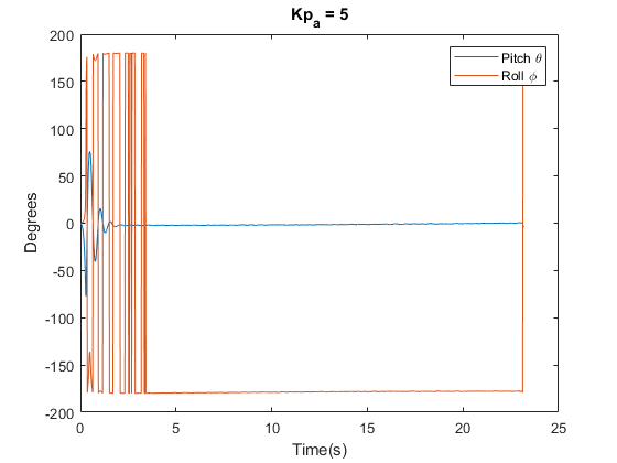
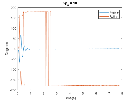
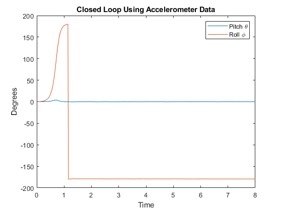
With K_p = 10 and K_i = 0.5, the sensor was placed upside down to test convergence to a 180° rotation. The experimental responses were comparable to the MATLAB simulation, though the axes approached 180° from the opposite side.

Actual closed loop feedback — Fig 17: Experimental closed loop accelerometer feedback

7. Conclusion

With calibration techniques and familiarization with DCM rotation matrices, attitude sensors are now well understood. There are several approaches to accomplish this, including using the TRIAD algorithm vs. the closed loop feedback system explored here. Attitude sensors can be accomplished in many ways — this is just one version of an implementation using complementary feedback filtering.

References

[1]Ladislav, B., Pavel, C. & Martin, D. (2014). "Navigation of robotic platform with using inertial measurement unit and Direct Cosine Matrix." Proceedings ELMAR-2014.

[2]Welch, G. & Bishop, G. "An Introduction to the Kalman Filter."

[3]de Marina, H. G. et al. (2012). "UAV Attitude Estimation Using Unscented Kalman Filter and TRIAD." IEEE Transactions on Industrial Electronics, vol. 59, no. 11, pp. 4465-4474.