Walker: A Simple Millipede Bot
Using biological inspiration from millipedes and centipedes, this thesis develops a cost-effective and easily reproducible robot design for traversal through diverse terrain.
B.S. Robotics Engineering · Supervised by Prof. Steve McGuire · Dept. of Electrical and Computer Engineering
Abstract
Within the field of robotics, there is a demand for robots capable of atypical terrain traversal. Atypical environments like stairs, rocky trails, and off-road locations consist of chaotic, non-flat terrain that ordinary wheeled robots struggle to cross. Companies like Boston Dynamics have developed humanoid and animal-like robots capable of traversing such terrain; however, these robot designs are expensive and complicated.
Using biological inspiration from millipedes and centipedes, this paper develops a cost-effective and easily reproducible design to solve the problem of traversal through diverse terrain. The development included research into the biology of millipedes and centipedes, a review of existing literature on insect-inspired leg actuators, implementation of an existing cam actuator by Wan and Song, and development of a simulation environment tested by hardware implementation — all completed at home in novel, affordable ways due to the COVID-19 Pandemic.
1. Introduction
1.1 Problem Statement
The need for robots capable of maneuvering uneven terrain grows yearly as simple wheeled robots are often limited in their ability to traverse non-flat surfaces. The field of bio-locomotive design looks to nature for inspiration, treating animals as robust, dynamic movement systems evolved precisely for their habitat.
Existing studies have investigated the particular robust locomotive characteristics of millipedes and centipedes as motivation for solving chaotic terrain traversal.
Though previous papers have attempted to recreate omnipede platforms by emulating millipede behavior, the resulting designs often use numerous motors for each body segment and complicated control schemes, decreasing the ease of reproduction. Walker aims to build a simplified omnipede robot that utilizes the advantageous characteristics of the Myriapoda subphylum while keeping fabrication simple and affordable.
These many-legged insects cross diverse habitats and present a simple, easy to emulate, and highly modular body structure. My research expands upon present analytical literature on the locomotive mechanisms of millipedes and centipedes as robotic inspiration.
1.2 Existing Work
Several researchers have explored multi-legged robots inspired by myriapods. Key sources that informed this work include:
- “Millipede-Inspired Locomotion for Rumen Monitoring through Remotely Operated Vehicle” by Garcia [7]
- “Centipede Robot for Uneven Terrain Exploration” by Koh et al. [10]
- “Decentralized control mechanism underlying interlimb coordination of millipedes” by Kano et al. [9]
- “The Kinematic Design of the OmniPede” by Long et al. [11]
Garcia provided an extensive analysis of millipede gait kinematics, validating the cycloid trajectory model through After Effects video tracking of live specimens. Koh et al. developed a centipede robot for uneven terrain exploration using multiple servos per segment. Kano et al. investigated decentralized control mechanisms underlying interlimb coordination. Long et al. designed the OmniPede using geared bar mechanisms for leg actuation. Each of these designs, however, required multiple actuators per segment, increasing cost and complexity.
Garcia's personal correspondence was an excellent source of guidance, and his 2015 dissertation was the primary source for millipede locomotion investigation. His After Effects-based analysis of live millipede footage demonstrated that leg tips trace a circular arc during the transfer phase, providing the kinematic foundation that Walker's design builds upon.
1.3 Characteristics of a Millipede
Throughout the paper, the Myriapoda is referred to when referencing the insect species. The term omnipede is a placeholder for all abstracted robots that imitate the Myriapoda.
Myriapoda translates to “many-legged ones” and encompasses both millipedes (Diplopoda) and centipedes (Chilopoda). Foundational surveys by Manton, Hopkin et al., Wilson, and Minelli provide the biological basis for understanding myriapod locomotion and anatomy.
Regarding the research goal of developing a simple robot platform, the critical difference between these subgenera is leg motion. Millipede leg trajectory has been modeled along a geometrically simple, 2-axis trajectory with relative accuracy. The millipede's body suspends statically in the air as it moves forward. In contrast, the centipede's gait involves complexity in leg movement and lateral oscillatory body movement. The static body and leg movement of the millipede make it the primary inspiration for research.
Both insects incorporate a wave-like motion that propagates through the legs when traversing. This wave-like phenomenon is an effect of metachronal gait. A metachronal rhythm is not a Myriapoda-specific gait pattern, but in the Myriapoda, it manifests through a sequential movement of legs. Kano et al. reviewed metachronal gait through study and production of a closed feedback millipede robot. The metachronal wave propagating through the right and left side of millipede legs are in phase with each other, while the centipede's traveling waves are 180° out of phase. This difference in phase and lateral undulating locomotion causes most centipedes to move faster than millipedes. However, what the millipede lacks in speed, it compensates in thrust capabilities for burrowing.
1.3.1 Leg Anatomy
Manton's foundational analysis of arthropod locomotion showed that while millipede legs contain many segments, they are mostly rigid and can be simplified to a single rotating segment for modeling purposes. Fig. 1.2 shows the many leg structures that the Kentish Pin-head Millipede has, but Manton notes that most add no further motion and are almost entirely rigid. The leg motion occurs primarily in a 2D plane perpendicular to the body axis, which greatly simplifies the kinematic model.
With many segments across a single leg, the trajectory of each leg occurs across all three positional axes. In other words, a single motor-controlled actuator cannot precisely emulate the trajectory. Notwithstanding, the trajectory can be mostly represented with simple kinematic equations.
1.3.2 Gait Analysis
Millipede locomotion is governed by duty cycle modulation, ranging from 0.3 to 0.7. The duty cycle D represents the ratio of propulsive (ground contact) time to total stride period. Low duty cycles (~0.3) produce a “high gear” mode optimized for speed, while high duty cycles (~0.7) produce a “low gear” mode optimized for thrust and burrowing force. The legs move in a metachronal wave — a sequential ripple pattern where each leg lifts only when neighboring legs are on the ground to provide support.
Manton recognized gait shift in backstroke/forward-stroke analysis. Garcia found that the duty cycle is the same across all legs and that the millipede does little to change angular velocity. The 6:4 ratio represents the time legs spend in forward stroke to backstroke. The phase difference between neighboring legs is also affected by duty cycle shift. The wavelength of the metachronal wave is a more apt description of the changing dynamics of millipede gait. The comparison between legs in backstroke to forward stroke — the ratio of legs in propulsive state to transfer state — is an effect of the changing metachronal wave.
1.3.3 Why Millipedes?
Millipedes maintain a constant body length throughout their gait, making them relatively easy to mimic with rigid body materials. Their body suspends statically as it moves forward — unlike centipedes, which exhibit lateral oscillatory body movement. Both species use metachronal waves, but with a key difference: millipede left/right waves are in phase, while centipede waves are 180° out of phase, producing lateral undulation.
The entirety of its gait modulation is due to the characteristics of the metachronal wave propagating through its legs. Considering that the millipede maintains a rigid body structure throughout its gait and can maneuver across varied environments, it presents a system with great potential for robotic emulation.
Left and right metachronal waves are in phase. Body remains rigid. Optimized for thrust and burrowing.
Left and right waves are 180° out of phase with lateral body undulation. Optimized for speed.
2. Kinematic Model
Before producing an omnipede robot, this chapter surveys the existing literature on millipede motion and derives a system of kinematic equations for modeling the movement of the Walker robot. The kinematic model describes the motion of omnipedes to be mimicked by Walker, independent of inertial considerations. Reviewing the academic literature did not reveal any system of dynamics equations for modeling these metachronal wave-based insects, so Chapter 4 considers the dynamics of motion using a 3D simulation developed in Matlab.
2.1 Literature Review
Despite the simplicity of leg motion, the kinematics of the metachronal wave proves to be rather complex. The Myriapoda constantly shifts its metachronal gait to traverse diverse geography. Kano et al. developed a complicated multi-motor, multi-sensor robot but his approach focused on actuation through feedback rather than kinematic description. Creating a complex robot is beyond the scope of Walker. Since there exists no uncomplicated kinematic model for metachronal rhythm, the analysis is reduced to a primarily qualitative description.
The kinematic model is based on three simplifying assumptions from Sathirapongsasuti et al.: the number of leg segments is one, every leg shares a common motion pattern, and the tip of each leg traces a circle of reference. When walking on a surface, this circle is trimmed to a segment, creating a cycloid trajectory split into two distinct phases.
As described in Section 1.3.1, the legs of a millipede can be modeled on a two-dimensional plane and assumed to maintain the same trajectory. Other studies explored this reductive model and garnered working locomotive robotic systems. This simplified kinematic system is shown to be effective by Koh et al., Garcia, and Long et al.
2.1.1 Kinematics of Leg Motion
The model rests on three simplifying assumptions from Sathirapongsasuti et al.:
- The number of millipede leg segments is one
- Every leg shares a common motion pattern
- The tip of each leg traces out a circle (circle of reference)
In the transfer phase, the leg lifts off the ground and swings forward along a circular arc. In the propulsive phase, the leg contacts the ground and pushes the body forward along a straight line. The position equations describe x(t) and y(t) for each phase, parameterized by the duty cycle D = ttransfer / tpropulsive.
Garcia validated this model by tracking live millipede footage in After Effects, overlaying the theoretical cycloid trajectory onto the tracked leg positions. The fit confirmed the circle-of-reference model is representative of real millipede motion.
This model for the leg trajectory is standard in bio-inspired robot design and is often used in robotics to describe any poly-pedal system. The half-circle trajectory of the foot traces out a cycloid when moving forward.
The time phase between adjacent legs is τt = d / Vwave. The relationship between transfer and propulsive periods determines most characteristics once the reference circle radius is set.
Core kinematic equations derived from the circle-of-reference model. R is the reference circle radius, θ is the arc angle, and t_T / t_p are the transfer and propulsive period durations.
The duty cycle D = t_transfer / t_propulsive determines the wave characteristics and thrust behavior, ranging from 0.3 (high speed) to 0.7 (high thrust).
2.1.2 Qualitative Understanding of Metachronal Gait
Garcia et al. showed that the metachronal gait specific to millipedes makes them highly capable of burrowing. Kano et al. also studied metachronal wave characteristics, focusing on bio-sensory feedback systems.
The metachronal wave can be modulated for different purposes. Higher duty cycles increase the number of legs on the ground at any time, generating more thrust — Garcia noted this is the mode used during burrowing. Lower duty cycles reduce ground contact time per leg, increasing stride frequency and speed. The lower duty cycle gait creates greater velocities for the millipede, in contrast to the higher duty cycle gait that produces greater thrust and lower speed. This modulation is achieved purely by varying the duty cycle parameter, making it straightforward to implement in a robotic system with a single control variable per leg pair.
3. Design
The broad design goal of Walker is to create a straightforward simplified omnipede robot. Due to the limitations driven by the COVID-19 pandemic, research avoided development beyond leg mechanisms. This chapter is dedicated entirely to researching leg mechanisms as a basis for the Walker robot build and simulation.
To create a simple millipede-like robot, a novel and reproducible leg is necessary. Existing leg actuators in the academic literature were analyzed, improved upon, and 3D modeled in Fusion 360 for manufacturing analysis. The design goals were: a single actuated leg with one degree of freedom, minimized individual parts to fewer than three, and a foot path creating the half-circle trajectory described in the kinematic model.
The scoring rubric compares the number of parts, whether the device creates the desired trajectory, and a non-rigorous fault score for additional issues. Parts score: 5 if fewer than 3 parts, minus 1 per additional part. Trajectory score: flat 5 if the desired half-circle is met, 0 otherwise. The categories are summed and then the fault score is subtracted.
The Kano et al. design is too complex for Walker — Kano's research focused on control theory actuation over design simplicity. The Koh et al. design focused on design simplicity using fixed rigid legs, but features little gait modulation. The investigation begins between the complexity of the Kano design and the simplicity of the Koh design, with the design of Long et al.
Geared Bar Mechanism (Long et al.)
The first mechanism is derived from Long et al., with similarities to 4-link and 5-link drive mechanisms. The benefit of this construction is its simple two-gear, single-motor design. Assuming constant angular velocity ω, the angular position of the drive gear is θ(t) = ωt. Each gear has a peg distance d from the gear's radius, with the leg position P derived from the peg positions C₁ and C₂.
Trajectory analysis with leg length L = 5 revealed significant deviation from the desired half-circle path. A longer leg length results in a flatter curve during the propulsive state, but the shape still doesn't meet the desired trajectory. All parts were 3D printed, restricting contours smaller than 0.5mm — greatly reducing the number of teeth these gears can possess. For this reason, the fault score is −2 points.
| Criterion | Score |
|---|---|
| Parts (3 parts, target <3) | 4/5 |
| Trajectory match | 0/5 |
| Faults (gear printing difficulty) | -1 |
| Total | 3/10 |
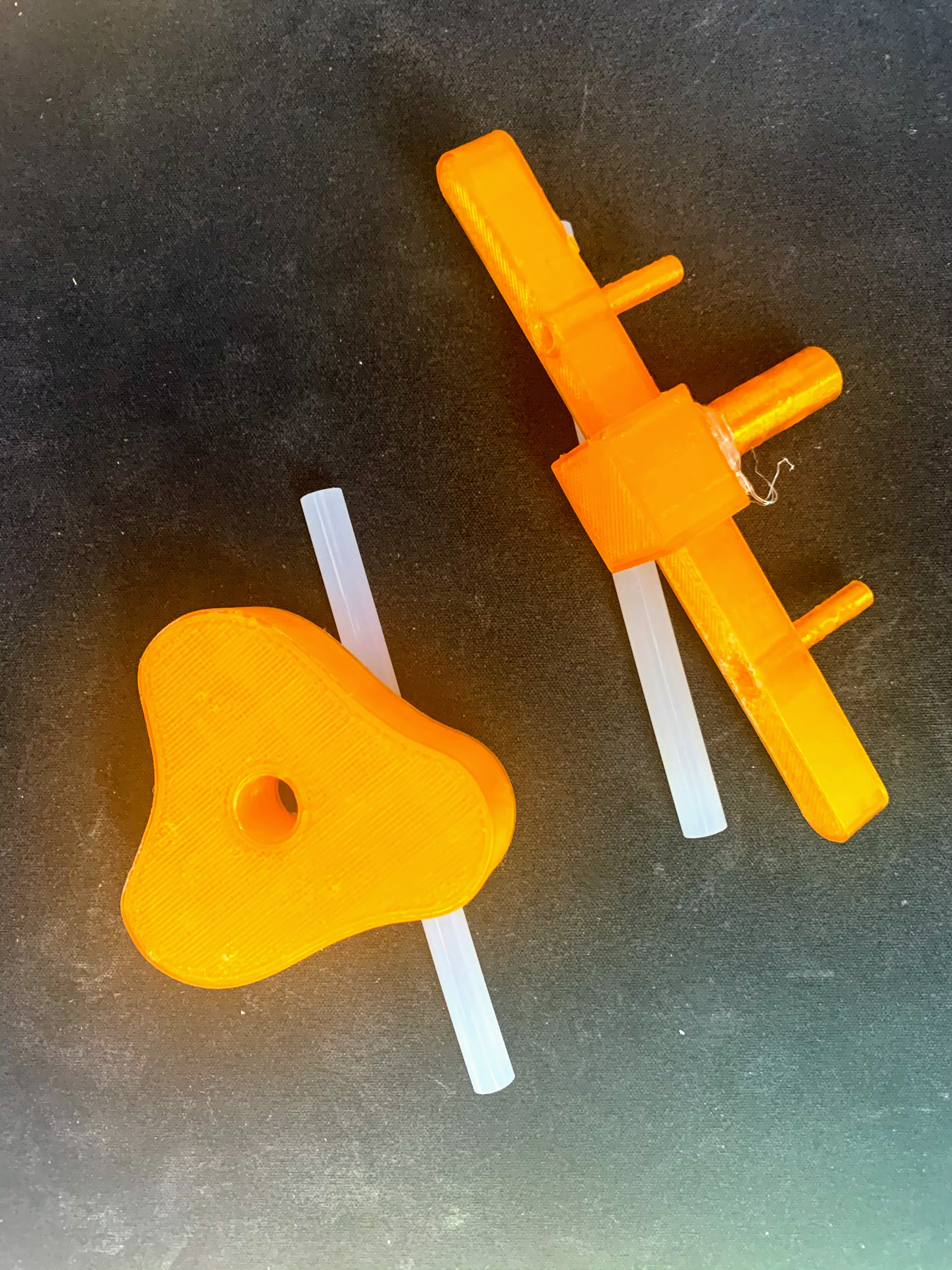
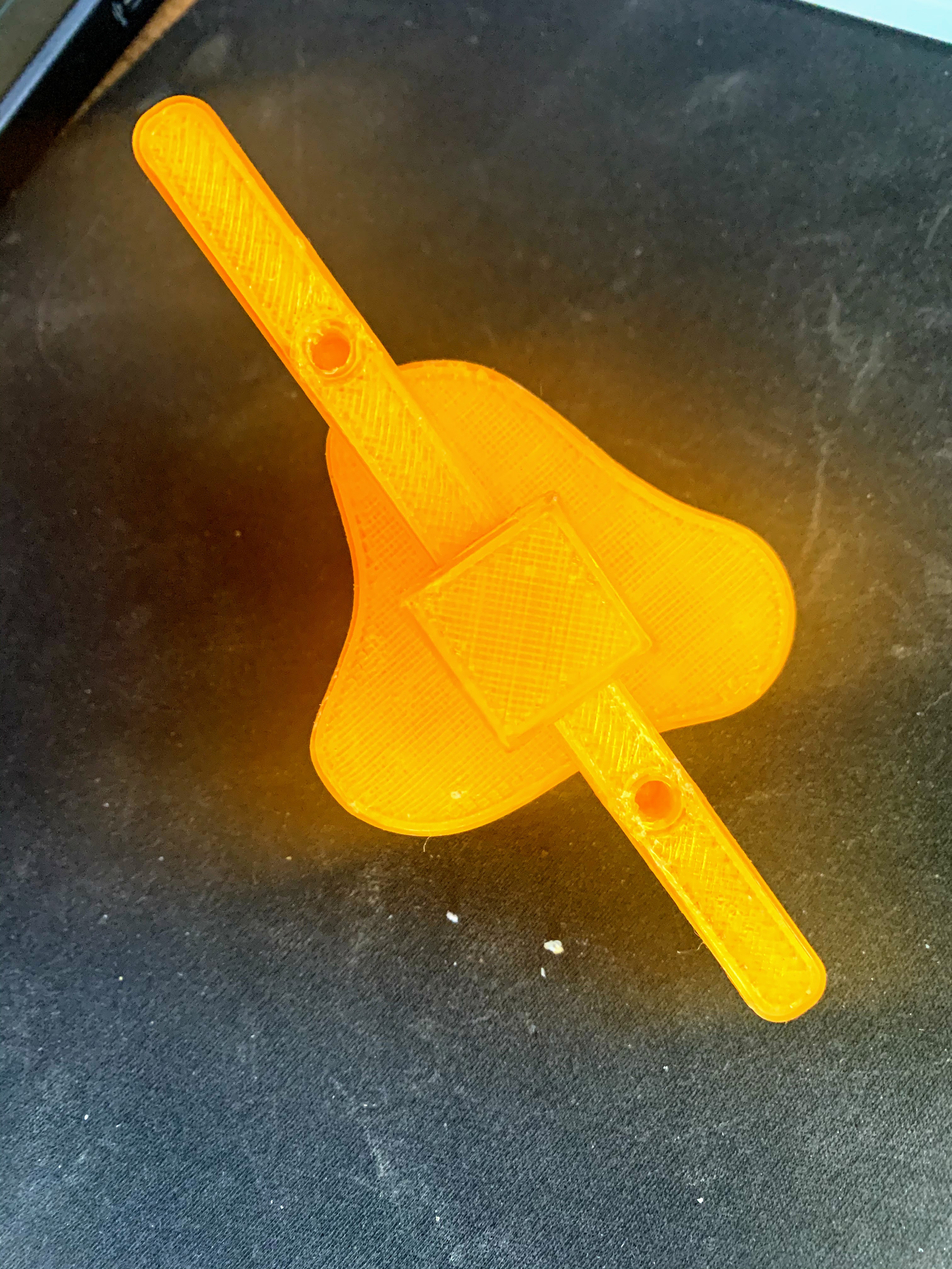
Custom Sliding Cam (Original Design)
Garcia et al. derives a cam actuator based on the design suggested by Wan & Song, which defines a cam shape that creates a half-circle trajectory. This cam design was also investigated by Crow in a mechanical engineering dissertation. Garcia's design modifies the Wan & Song design in favor of a single rotating leg, while Crow follows the original actuator more closely. Due to the complexity of the cam shape, I first developed an original mechanism inspired by Garcia's design.
This device was developed myself. The mechanism is an intuitive design that translates the trajectory path of the inner cam shape down by the length of the leg — the cam shape is the exact trajectory of the foot, translated by the leg length. The device can support a leg of any length and a cam of any shape, given low jerk (no curves too sharp), making it exceptionally intuitive to get the desired trajectory without much calculation.
The pitfalls include excessive friction points — the sliding joint and the peg that fits into the cam shape are two major friction sources. Secondly, a large amount of torque is pressed on the pin slot if the interior cam shape is too narrow. These combined factors lead to a fault score of −3. With 4 parts vs. the target of fewer than 3, other actuation devices were investigated.
| Criterion | Score |
|---|---|
| Parts (4 parts, target <3) | 3/5 |
| Trajectory match | 5/5 |
| Faults (friction, complexity) | -2 |
| Total | 6/10 |
Fixed Bearing Cam (Wan & Song)
The third and final mechanism is the most closely related implementation of the cam design from Wan & Song. The assembly includes a rotating link with bearings at a fixed distance and a sliding joint with leg attachment. The cam shape maintains a constant width d through rotation and is symmetrical about the Y axis — a single function f(θ) describing the shape from 0° to 90° defines the entire profile.
The cam shape is prescribed by four quadrant equations: S₁ = f(θ) for 0°–90°, S₂ = f(π−θ) for 90°–180°, S₃ = d−f(θ−π) for 180°–270°, and S₄ = d−f(2π−θ) for 270°–360°.
The cam profile is derived from: since the upper half creates a straight-line trajectory at height −H, we get R = −H/sin(θ), and S₁ = f(θ) = (L + d)/2 − H/sin(θ). The minimum theoretical angle λ = arcsin(2H/(L+d)) defines where the function goes to negative infinity.
The variable α defines an angle arbitrarily greater than λ as a smoother connection point, from which it would be impossible to create a smooth curve directly from λ. Iterative testing for smooth cam curves determines α. Refer to Conte and De Boor for inspiration on polynomial approximations and interpolation.
Crow finds that choosing an angular span of 60° maximizes the axle height H, bearing width d, and span. Initial parameters were H = 0.43L, d = 0.195L, but the initial curve fittings produced shapes too sharp at θ = 90°. To reduce this jerk motion, a wider diameter of d = 0.4L was determined through trial and error. Crow's axle height and bearing width values were a point of reference, but further iterative analysis on Matlab yielded the final values.
To smoothly connect the upper and lower cam profile, polynomial spline interpolation is required. Wan & Song suggests a sixth-order polynomial; Crow uses a fourth-order. The final design usesMakima polynomial spline interpolation for smooth transitions. Unlike the original proposed shape, the final design removes the exterior follower wall in favor of a single interior cam shape with a rotating armature. The mechanism's only fault is the torque forces near the vertical position, garnering a fault score of −1.
| Criterion | Score |
|---|---|
| Parts (3 parts, target <3) | 4/5 |
| Trajectory match | 5/5 |
| Faults (minor print tolerance) | 0 |
| Total | 9/10 |
Cam Profile Development
The cam profile went through multiple iterations: initial derivation from kinematic equations, refined angular span optimization, and finally Makima spline smoothing. The resulting profile produces a trajectory validated against the ideal half-circle path.
3.2 Conclusion
The design evolution progressed from Long's geared bar mechanism through an original sliding cam to the final Wan & Song fixed bearing cam. The final 3D model is robust yet straightforward — the mechanism creates the desired half-circle foot trajectory, the number of separate parts is 3 (pegs are considered part of the leg), overall friction is decreased, and the parts are large enough that print resolution can be coarse (> 0.5mm).
| Design | Parts | Trajectory | Faults | Overall |
|---|---|---|---|---|
| Gear Mechanism (Long) | 3 | No | −2 | 5/10 |
| Slide Cam (Original) | 4 | Yes | −3 | 6/10 |
| Cam Mechanism (Wan & Song) | 3 | Yes | −1 | 9/10 |
4. Simulation
This chapter strays from simply mimicking millipede motion and focuses on maximizing the stability of the robot design based upon the developed cam actuator. My analysis recognizes the thrust benefits of millipede motion but focuses on stability rather than speed or thrust potential. Garcia's study of millipede locomotion further explores the thrust benefits. An understanding of the stability of the system proves its efficacy, which future studies can then modulate for a specific analysis of insect gaits.
4.1 Kinematic Equation Analysis
Before running full dynamics simulations, a kinematic analysis was performed to narrow viable gait configurations. The goal was to maximize ground contact time — the fraction of the gait cycle where at least one leg per side touches the ground. Centipede-like motion (180° phase offset between left and right legs) was found to significantly reduce no-contact time compared to millipede-like motion.
The cam actuator is two-sided, meaning each leg device draws out two cycloids 180° out of phase with each other.
The Simscape environment takes upwards of fifteen minutes per simulation to compile and run.
| Leg Pairs | Phase Diff | Millipede | Centipede |
|---|---|---|---|
| 2 | 0° | 3.14s | 1.56s |
| 2 | 30° | 2.10s | 0.00s |
| 2 | 60° | 1.05s | 0.00s |
| 2 | 90° | 1.56s | 1.56s |
| 3 | 0° | 3.14s | 1.56s |
| 3 | 30° | 1.05s | 0.00s |
| 3 | 60° | 0.00s | 0.00s |
| 3 | 90° | 1.56s | 1.56s |
| 4 | 0° | 3.14s | 1.56s |
| 4 | 30° | 0.52s | 0.00s |
| 4 | 60° | 0.00s | 0.00s |
| 4 | 90° | 1.56s | 1.56s |
| 5 | 0° | 3.14s | 1.56s |
| 5 | 30° | 0.00s | 0.00s |
| 5 | 60° | 0.00s | 0.00s |
| 5 | 90° | 1.56s | 1.56s |
| 6 | 0° | 3.14s | 1.56s |
| 6 | 30° | 0.00s | 0.00s |
| 6 | 60° | 0.00s | 0.00s |
| 6 | 90° | 1.56s | 1.56s |
Time (in seconds) with no ground contact over a 10-second simulation. Lower is better. Centipede configurations with 3+ leg pairs achieve zero no-contact time.
4.2 Simscape Multibody Simulations
4.2.1 Iterations
The simulation went through three generations of increasing fidelity. Gen 1 was a rough proof of concept validating basic forward motion. Gen 2 attempted to use the custom sliding cam but proved too complex to simulate reliably. Gen 3 adopted the Wan & Song cam design, enabling full dynamics analysis across multiple leg counts and gait configurations.
The development process with Simscape involved uploading the Fusion 360 bodies to Onshape.com and creating joint assemblies uploaded to Matlab.
The second generation removed the rotating component and simulated motion without that contact point, resulting in an inaccurate simulation.
4.2.2 Final Environment
The final Simscape environment consists of two reusable components: a body segment component (rigid body with mass properties) and a leg segment component (cam-driven joint with revolute and slider constraints). These components are parameterized and chained together to form configurations with varying leg counts and phase offsets.
The rotation of the leg is controlled by angular position values. The gait switcher adds a simple user interface for changing left and right leg ninety degrees out-of-phase.
A revolute joint and slider control the rotating arm constrained by a cam shape. A foot is attached to either side of the leg with four contact points for measuring ground contact.
Though features like exact body shape and center of gravity are not included, they are trivial to add in future work.
4.3 Results
Center of gravity (CoG) measurements across 10-second simulations revealed that the centipede 8-leg configuration was the most stable overall. Centipede gaits exhibited extreme vertical instability (large CoG oscillations in Y) but excellent horizontal stability (smooth, consistent forward progress). Millipede configurations moved slower with greater velocity variability. The centipede motion tends towards more chaotic swaying as well as drift but within a confined region. Of the tested locomotive patterns, the centipede motion with eight legs is the most stable.
Center of gravity measurements from 10-second simulations across four gait configurations with 60° phase difference.
Key finding: centipede locomotion with neighboring legs 60° out of phase provides the most stable system, with zero ground-contact-loss time for configurations with 3+ leg pairs. This creates greater stability with fewer legs, lowering the cost of the final robot.
The lack of physical modeling of the connections and body had a negligible effect on studying the stability of the system's gait dynamics.
4.3.1 Conclusion on Simulation
The analysis between the kinematics and the Matlab simulation corroborate the conclusion that centipede locomotion with neighboring legs 60° out of phase provides the most stable system. The simulation environment is capable of measuring torque on each leg actuation joint, the speed of the robot, and providing a test harness for different body shapes.
5. Final Model & Conclusions
Two design iterations were printed and attached to an Antrader Dual Shaft 3-6V Motor for testing.
5.1 Print Faults & Fixes
The cam mechanism was 3D printed using a Raised 3D Pro2 printer at 0.5mm precision with ideaMaker as the slicer. The first print iteration revealed three faults: an unstable shaft connection (too narrow at the base), no mounting brackets for motor attachment, and sharp contour edges causing print head jerk. The second iteration addressed all three by widening the shaft base, adding bracket geometry, rounding sharp edges, and reducing infill to lower print time.
To reduce print time, the interiors of the shapes contained several cardboard-like edges, in place of a complete infill, which negligibly affected stability.
5.1.1 Conclusion on Print
Other manufacturing processes could avoid the issues that printing created. Crow manufactured a similar device using metal, which might be more promising for build stability. Another approach would use multiple materials — 3D plastic for the cam, metal for the rotary arm and legs. Widening the base of the rotary arm shaft created a more stable connection. Rounding the contours improved print quality consistency. The only remaining design consideration is frictional contact between the leg ends and ground — cursory testing showed improvement with glued rubber pieces.
5.2 Testing
The objective of testing the leg mechanism with a limited budget is to acquire experimental data compared to the simulation data. Comparable data experimentally proves the developed Simscape Multibody simulation environment concerning the type of data obtained, i.e., gait dynamics.
5.2.1 Home-Brew vs. Ideal
Due to COVID-19 pandemic restrictions, no lab equipment was available. All testing was performed at home using consumer hardware and Adobe After Effects as the primary measurement tool — a technique borrowed from Garcia's biological analysis work.
Ideally, the relative angular position would be sensed with a quadrature encoder attached to the back arm of the motor. Kano's test environment mounted a motor above a conveyor belt capable of measuring thrust potential.
5.2.2 Testing Trajectory
An Arduino-based test harness drove the cam mechanism with a DC motor. A potentiometer measured angular position, and a voltage divider circuit controlled motor speed for consistent test conditions.
The test system is comprised of an Arduino Uno, a 10-spin potentiometer for angular position detection, and a potentiometer in a voltage divider circuit to control the speed of the DC motor.
The trajectory was measured using After Effects motion tracking of slow-motion video. This motion data does not include any time data, as an iPhone 8s with custom slow-mo software captured the video. This issue hinders capturing angular velocity.
5.2.3 After Effects Analysis
Slow-motion video of the cam mechanism was tracked in After Effects to extract the foot tip trajectory. The tracked data confirmed the designed 60° propulsive ground contact span. Normalized position data was overlaid on the ideal trajectory, yielding a maximum error of 4.6mm — well within acceptable tolerances for the target application.
Typically, cameras record at a standard rate of 30 frames per second (fps), or possibly 60 fps, but the iPhone uses software that automatically slowed down parts of the video and added inconsistencies in using the frames as a determination of time.
After Effects motion-tracked a green dot on a piece of paper attached to the foot of the cam for one rotation.
Analysis ignored velocity as tracking data returns position based on frame data, not time data, because of the custom iPhone slow-motion capture.
Angle is determined with trigonometry: θ = arcsin(y_pos/x_pos).
The home laboratory provides pixel data; the trajectory is normalized to the known leg length of 120mm.
The maximum error of 4.6mm occurs between 70 to 120 degrees at the bottom of the foot trajectory. Minor improvements would include a better mounting surface and larger pegs — the pegs used were shorter than the cam width and tended to skew.
5.2.4 Failed Tests
5.2.4.1 Potentiometer
The potentiometer produced extremely noisy angular position data; even after applying 80Hz and 15Hz low-pass filters, the signal remained too noisy for precise trajectory reconstruction.
An attempt was made to reduce high frequency noise with an RC low pass filter as well as a running average.
The 15Hz cutoff filter shows near linearity at turns below approximately 500 degrees. From a line of best fit, the approximate angular velocity is -395.325°/second.
5.2.4.2 IMU
The IMU (MPU9250) suffered from integration drift, making linear position data completely unusable for trajectory validation.
An IMU was attached to a piece of long construction paper held below the mounted, rotating leg. When in contact, the leg pushed the paper like a conveyor belt.
Using the accelerometer on the MPU9250 with the highest polling rate, integrated accelerometer data found the paper's position on a single axis (X_pos = ∫∫&xdot;). However, integration of inaccurate data creates huge errors.
The sensor was held on a level surface and slowly dragged forward and backward. Accurate data should return position to zero at origin, but inaccuracy prevents this.
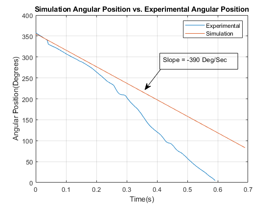
5.2.5 Simulation vs. Actual
Despite the sensor failures, the After Effects trajectory analysis provided sufficient validation. The simulation was confirmed, and the device functions within a negligible margin of its intended design.
Fig 5.14 shows a cursory observation of angular position vs time. The frame rate of the camera might be variable, so this data should not be considered with complete confidence. The simulation data is linear while the actual device drifts from linearity. Testing captured these data sets while the mechanism was suspended in the air, restricting any ground contact.
5.3 Conclusion & Future Work
This thesis contributes a literature review of omnipede gait kinematics, a verified Simscape Multibody simulation environment for omnipede robots, and a robust, affordable prototype of the Wan & Song cam leg actuator using modern 3D printing.
After considering several leg actuators, a novel, simple actuation device by Wan & Song emulating the idealized gait kinematics of the Myriapoda developed by Sathirapongsasuti et al. proved a robust leg mechanism for Walker. This paper contributes to robotics and mechanical engineering a simulation environment for omnipedes based upon Sathirapongsasuti's kinematic model verified by austere sensor technology.
In the observation of millipede vs. centipede locomotion through a literature review, studies like Manton, Garcia et al., and Kano et al. investigated the thrust potential of the former and the speed of the latter.
The simulation proved that centipede-like locomotion with 60° phase offset provides optimal stability, while the 3D-printed cam mechanism achieved the designed half-circle foot trajectory with only 4.6mm maximum error. The entire project was completed at home during the COVID-19 pandemic, demonstrating that meaningful robotics research can be conducted with accessible tools.
Crow's design lacked the double-sided leg of the source paper, as well as any simulation. In the future, this actuator could replace bulky multi-motored locomotive systems not limited to just millipede motion.
Future work includes: full-body Walker assembly with multiple cam-driven segments, expanded terrain simulation with obstacle geometries, force analysis with experimentally-verified friction parameters, and exploring this cam actuator as a general replacement for bulky multi-motor locomotion systems beyond millipede-inspired designs.